Predicting the Year a Song was Released [PyTorch]

PyTorch is a Pythonic implementation of a deep-learning library named Torch. PyTorch also includes support for C++ code. Originally developed at Facebook, PyTorch was released to the world in 2016.
In this article, we will first learn about a few distinguishing features of PyTorch. Next, we will use PyTorch to build a deep-learning model that can predict the year a song was released. The model will base its prediction on factors related to the tone, or timbre, of the corresponding singer.
Article Objectives
After reading this article, you should be able to
- describe the main features of PyTorch.
- obtain data that contains details about multiple songs.
- prepare the data for deep learning.
- create a deep-learning model using the prepared data.
- obtain a prediction from the model.
Let us begin with PyTorch features.
Describing the Main Features of PyTorch
PyTorch is open-source and facilitates fast numerical computing. To enable hardware acceleration for fast computing, PyTorch leverages graphics processing units (GPUs) if they are available.
Another distinguishing feature of PyTorch is that it lets you use dynamic computational graphs in deep-learning models. This feature made PyTorch a formidable competitor of TensorFlow 1, a popular deep-learning library that relies on static computational graphs.
Understanding a Computational Graph
A computational graph is a graphical representation of a mathematical equation. We can use a computational graph to represent the layer-based structure, or neural network, of a deep-learning model as well. This is because a neural network does, after all, perform mathematical calculations.
The Components of a Computational Graph
A computational graph consists of the following components:
Nodes: A node denotes a mathematical operation, such as addition.
Variables: Variables are of two types, inputs and outputs. Nodes process any inputs that they receive into outputs.
Connectors: A connector, which is also called an edge, connects a node to one or more inputs and an output.
Consider the equation \(ax^2 + bxy + cy^2 = d\). In this equation, \(x\) and \(y\) are variables; \(a\), \(b\), \(c\), and \(d\) are arbitrary constants; and \(a\), \(b\), and \(c\) are each non zero. Here is a computational graph of the equation:
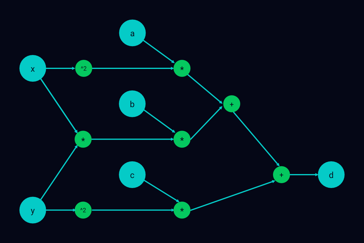
A computational graph of a quadratic equation
In the graph above, the bigger circles represent input variables and the final output, \(d\). The smaller circles are nodes, and the arrows, which link the bigger circles with the smaller circles, are connectors or edges.
The computational graph of a deep-learning model is not very different. The main components of this graph are described below:
Input variables: Any data that you supply to the model constitute the input variables.
Nodes: The nodes are the simple mathematical operations and error-handling and weight-adjusting functions that you apply to the input variables. The nodes are distributed across the layers of the corresponding neural network. All the nodes of a layer work together to generate an output for the layer.
Output variables: The output of each layer is an output variable.
Connectors: Just as in an ordinary computational graph, a connector of a neural-network graph connects a node to one or more inputs and an output.
What about static and dynamic computational graphs? Let us discuss them next.
The Difference Between Static and Dynamic Computational Graphs
The computational graph of a deep-learning model is said to be static if you define and freeze the nodes and control flow of the graph before you begin training the model. You cannot modify the graph during or after a forward or backward pass.
A dynamic computational graph does not impose such restrictions on you. You can change the nodes and control flow of the graph while you are training or running the model to which the graph pertains.
Dynamic computational graphs are useful for tasks such as natural language processing (NLP). Suppose you are processing a group of sentences using a deep-learning model. In this sentence-processing task, each input of a forward pass could contain a different number of words. So, each input could require a unique computational graph.
Defining and freezing all possible static graphs for the sentence-processing task can be effort intensive. Modifying input data at the beginning of each forward pass can also be tedious. A better alternative is to use a dynamic graph for this task.
You can create a model containing a dynamic graph using PyTorch. A PyTorch model generates a new dynamic-graph instance at the beginning of each of its forward passes. It configures the graph instance for a forward pass according to the amount and type of input data that is available to the pass.
A dynamic graph saves you from modifying each new batch of input data to fit the control flow of a model. However, dynamic graphs also have a drawback. Let us find out what this drawback is.
The Drawback of Dynamic Computational Graphs
A significant shortcoming of dynamic computational graphs is that you have to rebuild them each time you modify them. PyTorch optimizes the rebuilding process, but this process can still be somewhat time consuming. That’s why PyTorch lets you convert a dynamic graph into a near-static graph for production environments.
The benefits of PyTorch far outweigh its drawback. It can prove very handy in quickly prototyping and testing models. Let us validate this by working on the proposed project.
Building a Release-Year Predictor
I had outlined the project steps in the Article Objectives section. Here are the steps again:
- Obtain data that contains details about multiple songs.
- Prepare the data for deep learning.
- Create a deep-learning model using the prepared data.
- Obtain a prediction from the model.
Let us proceed to the first step of the project.
Step 1: Obtaining Data About Songs
UCI Machine Learning Repository, an online repository of University of California, Irvine, contains a song dataset that will serve our purpose. This dataset contains 91 columns. Here is a description of the dependent and independent variables of the dataset:
Dependent variable: The first column of the dataset, column 0, represents the dependent variable. The column lists the release years of multiple songs. The values in the column range from 1922 to 2011.
Independent variables: Columns 1–91 represent the independent variables. Among these columns, 12 list timbre averages of songs and 78 list timbre covariances.
The dataset is available as a compressed TXT file. To make this file usable in our project, we will perform the following tasks:
- Download the compressed TXT file.
- Unzip the file into a Google Drive folder.
- Convert the file into an easier-to-use dataframe using
pandas, a Python-based library. - Assess the contents of the dataframe by retrieving and displaying a few details from it.
- Save a copy of the dataframe so that we can easily obtain the original dataframe later, if required.
Here is how we will perform the tasks:
Task 1: Downloading the Compressed TXT File
To accomplish this task, create a new Google Colab notebook and save the notebook in a root-level folder named deep-learning. Then, run the following command in the notebook.
!wget https://archive.ics.uci.edu/ml/machine-learning-databases/00203/YearPredictionMSD.txt.zip &> /dev/null
The command that you just ran would have downloaded the compressed file in a dynamic, temporary location. If you reset the runtime environment of the notebook, the file will be deleted.
To avoid losing the file, we will move it to a static Google Drive folder in the next task. This folder will be at the same level as the project notebook. Once we have relocated the file, we will unzip and rename it.
Task 2: Unzipping the File into a Google Drive Folder
To accomplish this task, first make sure that Google Drive is connected to the project notebook. Then, run the following commands.
# Creating a folder for the unzipped file
!mkdir /content/drive/MyDrive/deep-learning/proj2_assets

# Unzipping the compressed file to the new folder
!unzip /content/YearPredictionMSD.txt.zip -d /content/drive/MyDrive/deep-learning/proj2_assets

# Renaming the unzipped file songdata.txt
!mv /content/drive/MyDrive/deep-learning/proj2_assets/YearPredictionMSD.txt /content/drive/MyDrive/deep-learning/proj2_assets/songdata.txt
Task 3: Converting the File into a Dataframe
We intend to convert the file and display information from it using the pandas library. So, first, we will import pandas and set display criteria for pandas output. Here is the code that we will use:
# Importing the pandas library
import pandas as pd

# Configuring display settings of pandas output
pd.set_option('precision', 3)
pd.set_option('display.width', 1000)
pd.set_option('display.max_rows', 500)
pd.set_option('display.max_columns', 500)
pd.set_option('display.float_format', '{:.3f}'.format)
Next, to avoid typing or copy-pasting the path to the file repeatedly, we will save the path in a variable. We will use the following code to do this:
BASE_PATH = '/content/drive/MyDrive/deep-learning/proj2_assets/'
Finally, to convert the file into a pandas dataframe, we will run the following code:
df = pd.read_csv(BASE_PATH + 'songdata.txt', header=None)
In the next task, we will verify that the dataframe contains the data that we want.
Task 4: Assessing the Contents of the New Dataframe
Let us first look at the first row of the dataframe. Run the following code:
df.head(1)
The column names in the output appear numerical. The following code corroborates this:
df.columns.dtype
As it is easier to work with column names that are in string format, run the following code to convert the data type of the column names.
# Converting the column names to strings
df.columns = df.columns.astype(str)
Next, for easy identification, rename column 0, which represents the dependent or target variable.
# Assigning the name target to column 0
df.rename(columns={'0': 'target'}, inplace=True)
In addition, add a prefix to each of the other column names.
# Prefixing col_ to the other column names
features = df.columns[~df.columns.isin(['target'])]
df.rename(columns = dict(zip(features, 'col_' + features)), inplace=True)
Now, let us view an excerpt from the updated dataframe and verify the changes that we just made.
df.head()
We will also look at a few other details using the following lines of code:
# Printing the number of rows and columns of df and
# determining the number of null values
df.shape, df.isnull().sum().sum()
# Obtaining a statistical description of the data in df
df.describe()
# Listing the unique data types in df and
# the number of columns of each data type
df.dtypes.value_counts()
The dataframe seems complete and ready for further processing, so let us move on to the final task of this step.
Task 5: Saving a Copy of the Dataframe
We will convert the dataframe to the binary Feather format and save it in Google Drive. The Feather format will ensure that each column of the dataframe retains its data type. Here is the code that we will use:
df.to_feather(BASE_PATH + 'df_original')
Now, let us proceed to the second step.
Step 2: Preparing the Data for Deep Learning
In this step, we will separate the target column from columns 1–90 of df. Then, we will standardize the values in columns 1–90.
Standardization is necessary because the values in columns 1–90 have different ranges. The range variations can mislead our model about the importance of these columns. Standardization will rescale all the values and so remove ambiguity.
After we have standardized columns 1–90, we will split them, as well as the target column, for training and testing.
I have organized the requirements of this step into the following tasks:
- Separate the
targetcolumn from columns 1–90. - Standardize the values in columns 1–90.
- Create training and testing datasets using columns 1–90 and the
targetcolumn. - Save the training and testing datasets for later access.
Here is how we will perform these tasks:
Task 1: Separating the target Column from Columns 1–90
We will begin this task by importing the original version of the dataframe, which we had saved as a Feather file in the previous step. We will also verify that the dataset contains correct data. You can avoid these preliminary actions if the runtime environment of your notebook hasn’t been reset.
# Importing the saved dataframe
df = pd.read_feather(BASE_PATH + 'df_original')

# Verifying that the dataframe contains the right
# data: strings as column names and valid values
print('-'*31)
print(f'Data type of df columns: {df.columns.dtype}')
print('-'*31)

df.head(1)
Next, we will shuffle all the rows of df. Then, we will save columns 1–90 in a dataframe named X and the target column in a data series named Y.
seed = 123
df = df.sample(frac=1, random_state=seed)

X = df.iloc[:, 1:]

Y = df.iloc[:, 0]
In the code above, the frac=1 argument ensures that all the rows of the datasets are shuffled and returned.
Task 2: Standardizing the Values in Columns 1–90
Here is the code that we will use to standardize the values in X, which contains columns 1–90, and then view an excerpt from X:
# Standardizing X
X = (X - X.mean())/X.std()

# Printing the first five rows of standardized X
X.head()
Task 3: Creating Training and Testing Datasets
To split X and Y for training and testing, we will use the train_test_split function of sklearn. We will also view the shapes of the newly created datasets and then reset the indexes of the datasets.
# Splitting the datasets

from sklearn.model_selection import train_test_split

X_train, X_test, y_train, y_test = train_test_split(X, Y, test_size=0.025, random_state=seed)

# Printing the shapes of the new datasets
X_train.shape, y_train.shape, X_test.shape, y_test.shape
# Writing a function to reset the indexes of the new datasets
def reset_df_index(train, test):
  train.reset_index(drop=True, inplace=True)
  test.reset_index(drop=True, inplace=True)

# Resetting the indexes
reset_df_index(X_train, y_train)
reset_df_index(X_test, y_test)
Task 4: Saving the Training and Testing Datasets
Some of the datasets are dataframes and some are series objects. We will save the dataframes as feather files and the series objects as pickles. Here is the code that we will use:
X_train.to_feather(BASE_PATH + 'X_train')
y_train.to_pickle(BASE_PATH + 'y_train')
X_test.to_feather(BASE_PATH + 'X_test')
y_test.to_pickle(BASE_PATH + 'y_test')
Now that we have prepared the data, we can proceed to the next step.
Step 3: Creating a Deep-Learning Model Using the Prepared Data
In this step, we will perform the following tasks:
- Enable GPU use.
- Import relevant data and libraries.
- Make the data compatible with PyTorch.
- Initialize a deep-learning model.
- Initialize a loss function and an optimizer for the model.
- Train the model.
We will discuss relevant aspects of each task as we work through it. Let us begin with task 1.
Task 1: Enabling GPU Use
As we want fast processing, we will set GPU as the hardware accelerator for the project notebook. To enable GPU use, perform the steps listed below:
- On the menu bar at the top of the notebook, click Runtime.
- In the menu that opens, click Change runtime type.
- In the Notebook settings window that appears, from the Hardware accelerator list, select GPU and then click Save.
You can also watch a demonstration of these steps in the following video:
The process of changing the hardware accelerator resets the environment of a Colab notebook. This means that any data-containing variables are also reinitialized. We will take this into account in the next task.
Task 2: Importing Relevant Data and Libraries
We don’t need all the data that was available within the notebook before its environment was reset. We only require the training and testing datasets to proceed with the current and subsequent steps. We can easily retrieve these datasets from the feather and pickle files that we had saved at the end of the previous step. Here is code that will retrieve the datasets:
# Reading the feathered and pickled versions of the datasets
X_train = pd.read_feather(BASE_PATH + 'X_train')
y_train = pd.read_pickle(BASE_PATH + 'y_train')
X_test = pd.read_feather(BASE_PATH + 'X_test')
y_test = pd.read_pickle(BASE_PATH + 'y_test')
Next, as we want to build a PyTorch model, we will import the PyTorch library into the project notebook. We will also import the nn module of PyTorch, assigning the module a concise name. The nn module lets us easily create and train neural networks using predefined layers and functions.
# Importing the PyTorch library
import torch

# Importing the nn module
import torch.nn as nn
Finally, we will run the following code to verify that the Compute Unified Device Architecture (CUDA) package of PyTorch can leverage GPUs for faster processing:
torch.cuda.is_available()
The command above should return True.
Task 3: Making the Data Compatible with PyTorch
To make the training and testing datasets compatible with PyTorch, we will convert them into tensors in this task. A tensor is a basic building block of PyTorch code. A tensor stores a numerical value and can have 0 or more dimensions.
A zero-dimensional tensor, also called a rank 0 tensor, is just a scalar value. A rank 1 tensor is a vector-like structure (a one-dimensional array), a rank 2 tensor is a matrix-like structure (a two dimensional array—for example, a 2x2 or 3x3 matrix), and so on. Tensors can interact with and modify each other.
Here is code that will convert the datasets into tensors that can leverage GPU power:
# Ensuring that the tensors and any other
# PyTorch elements that we create for this project
# can use the GPU feature if it is available
if torch.cuda.is_available():
  device = torch.device("cuda")
else:
  device = torch.device("cpu")

# Converting the datasets into tensors
X_train = torch.tensor(X_train.values).float().to(device)
y_train = torch.tensor(y_train.values).float().to(device)
X_test = torch.tensor(X_test.values).float().to(device)
y_test = torch.tensor(y_test.values).float().to(device)
Task 4: Initializing a Deep-Learning Model
We will use the Sequential container of the nn module to initialize a deep neural network for our project. This network will consist of a sequence of four layers.
We won’t need to define the basic properties of the four layers. But we will have to specify the sizes of the inputs and outputs of each layer. We will run the following code to declare the sizes:
# Specifying the total number of independent variables
# in our data (i.e., the number of X_train
# columns) as the size of the input to the first layer
initial_input_size = X_train.shape[1]

# Specifying the number of features that the
# first layer should output
output_size_1 = 20

# Specifying the number of features that the
# second layer should output
output_size_2 = 10

# Specifying the number of features that the
# third layer should output
output_size_3 = 5

# Setting the size of the final output as 1 because
# we want only one release year predicted per song
final_output_size = 1
Now, we will initialize the model.
model = nn.Sequential(nn.Linear(initial_input_size, output_size_1),
nn.ReLU(),
nn.Linear(output_size_1, output_size_2),
nn.ReLU(),
nn.Linear(output_size_2, output_size_3),
nn.ReLU(),
nn.Linear(output_size_3, final_output_size))
The key elements of the initialization code are described below:
Linear: Part of thennmodule, theLinearclass helps us implement the layers of the neural-network model. EachLinearlayer in the initialization code above accepts two arguments. The first argument specifies the number of inputs to the layer and the second argument specifies the number of features that the layer should return.The first argument of the first
Linearlayer is the total number of independent variables in our sample data. From the secondLinearlayer onwards, the first argument of eachLinearlayer is the output size of its preceding layer.ReLU: Each of the first threeLinearlayers is followed by an activation layer,ReLU. AReLUlayer is an instance of theReLUclass of PyTorch.What does an activation layer do? It uses a function to modify the output of its preceding layer. In the case of a
ReLUlayer, this function is called a rectified linear unit (ReLU) function. A ReLU function returns a data element that it receives as is if the element is positive. It returns 0 if the element is negative.
After initializing the model, we must also shift it to the available GPU so that it can leverage GPU power. Run the following code to do this:
model.to(device)
That’s all there is to task 4. Now, let us proceed to the next task.
Task 5: Initializing a Loss Function and an Optimizer
We need a loss function to assess the prediction accuracy of our model and an optimizer to minimize prediction errors. The following are the elements that we will use to serve these purposes:
MSELoss: TheMSELossfunction of thennmodule will help us determine prediction accuracy.MSELosswill calculate the mean squared error (MSE) of the model. That is, it will indicate the difference between the actual release years of songs and the release years that the model predicts.Adam: For optimization, we will use theAdamalgorithm. This algorithm is part of theoptimpackage of PyTorch. TheAdamalgorithm can optimize model parameters (weights), thereby minimizing errors.To use
Adamwithin a model, we have to only pass on the weights that are associated with the model and a learning rate toAdam. It does the rest of the work for us.A weight is the importance that a layer of a neural network assigns to a feature of a sample dataset. A bias, by contrast, is an incorrect interpretation that a layer makes about a feature. And a learning rate is the rate at which an optimization algorithm adjusts the weights of a model to minimize errors.
Adamis more efficient than ordinary optimization algorithms because of three reasons. First, it maintains a separate learning rate for each weight of a model. Second, it continuously adjusts its learning rates, changing each learning rate independently of other learning rates. Third, it modifies a learning rate only in accordance with the weight that is associated with the rate and ignores all other weights.
Here is code that will initialize the MSELoss loss function and the Adam optimizer:
# Initializing MSELoss as the loss function
l_func = torch.nn.MSELoss()

# Initializing Adam
optimizer = torch.optim.Adam(model.parameters(), lr=0.01)
Task 6: Training the Model
We will use the following code to train the model:
| |
In the code above, we have chosen to train the model for 3500 iterations, using a for loop. You could change the number of iterations to, say, 3000 or 4000 and see how the model performs.
The purpose of each line of code within the for loop (lines 2–8) is described below:
- Line 2: Obtain a prediction from the model. Use the
squeezemethod to make the prediction one dimensional. - Line 3: Using the loss function,
l_func, that we had initialized earlier, determine the MSE of the prediction. - Line 4: Use the
zero_gradmethod ofAdamto remove any gradients inherited from the previous iteration. A gradient’s purpose is to improve prediction accuracy. It specifies the factors according to which the parameters of a model must change. We don’t want another iteration’s gradients affecting the current iteration, and so we should remove all non-native gradients. - Line 5: Use the
backwardmethod ofMSELossto calculate gradients for the current iteration. - Line 6: Run the
stepmethod ofAdamto modify weights based on the calculated gradients. - Line 7: Check whether the iteration number is divisible by 250.
- Line 8: If the condition in line 7 is satisfied, use the
itemmethod to extract the value in the output of the loss function. Also, display the value along with its corresponding iteration number.
Once we have trained the model, we can proceed to the final step of this project.
Step 4: Obtaining a Prediction from the Model
In this step, we will obtain predictions about specific songs in the test dataset. We will also display the actual release years (target values) of those songs as well as the predicted release years. We will run the following code blocks to do all this:
pred = model(X_test[4])
print("Actual value:", y_test[4].item(), "Predicted value:", round(pred.item()))
pred = model(X_test[2000])
print("Actual value:", y_test[2000].item(), "Predicted value:", round(pred.item()))
pred = model(X_test[35])
print("Actual value:", y_test[35].item(), "Predicted value:", round(pred.item()))
Conclusion
PyTorch is a deep-learning library that facilitates fast numerical computing. PyTorch leverages GPUs if they are available and lets us incorporate dynamic computational graphs in deep-learning models. If you want to build a deep-learning model wherein the inputs to each layer can vary, use PyTorch.
A significant drawback of dynamic computational graphs is that they have to be rebuilt each time they are modified. The rebuild process can take excess time. So, PyTorch allows us to convert dynamic computational graphs into near-static graphs for production environments, where time is of the essence.
Drawback notwithstanding, PyTorch works well for model prototyping and testing. For example, we can quickly build and test a deep neural network using the Sequential container of PyTorch. We have to specify only the type of class to use for each layer of the network (for example, the Linear class), the sizes of the inputs and output features of each layer, and the activation function to process the outputs of each layer. Sequential takes over from there and initializes the network.
To increase the prediction accuracy of a Sequential model, we train it in multiple iterations. During each iteration, we use a loss function, such as MSELoss, to assess the accuracy of the model. We also use an optimization algorithm, such as torch.optim.Adam to minimize errors.
Given its benefits and ease of use, PyTorch can be a good addition to your deep-learning knowhow. Try using PyTorch in your next deep-learning project.