Classifying Images Using Pretrained TensorFlow Models
Welcome to the first project in the Mastering Deep Learning Through Projects series. In this project, we will use pretrained TensorFlow models to classify images. Our goal is to understand how to use pretrained models and compare their accuracies.
Project Objectives
After completing this project, you should be able to
- explain the relevance of pretrained models.
- list three pretrained models.
- distinguish between the pretrained models.
- outline the process of using a pretrained model.
- obtain predictions from multiple pretrained models.
- compare the prediction accuracies of the models.
Download Code
All the project code is available in a Google Colab notebook.
Explaining the Relevance of Pretrained Models
Deep learning lets you use specialized algorithms to automatically obtain new insights and interpretations from data. And it works best with unstructured data, such as images, videos, and documents.
The accuracy of a deep-learning model usually depends on the amount of sample data it has been trained on. The more its sample data, the more accurate a model can turn out to be. However, training a deep-learning model from scratch on unstructured data can be a costly, resource-consuming process. That’s why pretrained models have become popular among deep-learning professionals.
Today, many pretrained models are available in the public domain or for small fees from cloud-service providers and other for-profit companies. Open-source deep-learning libraries like TensorFlow and PyTorch also include pretrained models.
A pretrained model is a ready-to-use model. It has already been trained on large amounts of data from a specific domain. It comes with a satisfactory level of prediction accuracy out of the box.
We can repurpose a pretrained model for a deep-learning project of the same domain without much effort. We won’t have to reinvent the wheel. We won’t have to spend too much time on model training. We can also avoid spending money on expensive computing resources.
To demonstrate the use of pretrained models through this project, I have selected three TensorFlow models. Let us get acquainted with these models.
Introducing the Three Pretrained Models
The keras module of TensorFlow 2 includes various pretrained models that can recognize objects in photos. From among these models, we will use ResNet50, DenseNet121, and DenseNet201 in this project.
What do the model names mean? Let us find out.
Decoding the Names of the Pretrained Models
An abbreviation and a numeric suffix compose the name of each pretrained model. Here is a description of these components:
Abbreviation: The abbreviation in a model name denotes the type of neural network on which the model is based. For example, ResNet50 is based on a residual neural network (ResNet). The other models that we intend to use, DenseNet121 and DenseNet201, have densely connected convolutional networks (DenseNets) as their foundations.
Numeric suffix: The number that is suffixed to a model name indicates the total number of layers in the model. ResNet50 contains 50 layers, DenseNet121 contains 121 layers, and DenseNet201 contains 201 layers.
The following figure highlights the components of the names ResNet50 and DenseNet121:
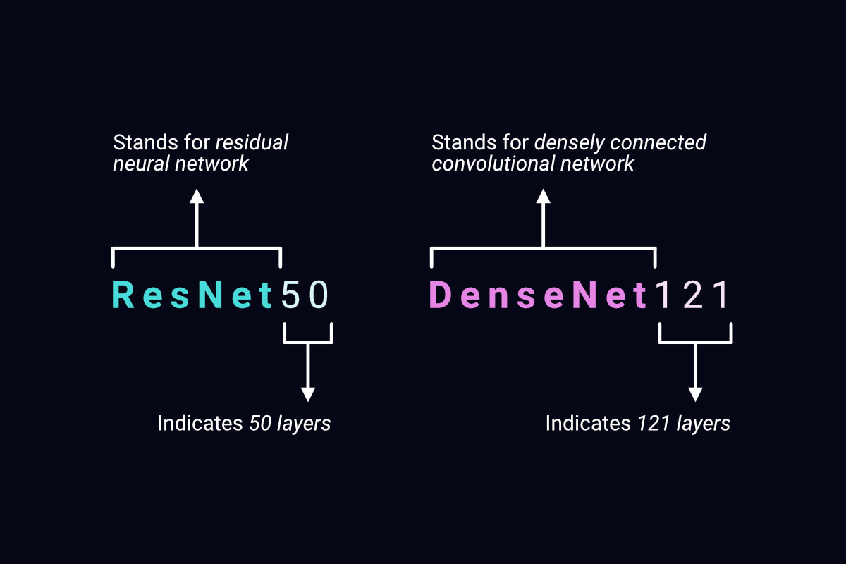
The components of model names
Next, let us find out how ResNets and DenseNets differ.
Distinguishing Between ResNets and DenseNets
In a ResNet model, each non-initial layer receives the output of only the layer that immediately precedes it. This output includes the features that the preceding layer had learned from the object that the model is processing.
The following figure is a representation of a ResNet:
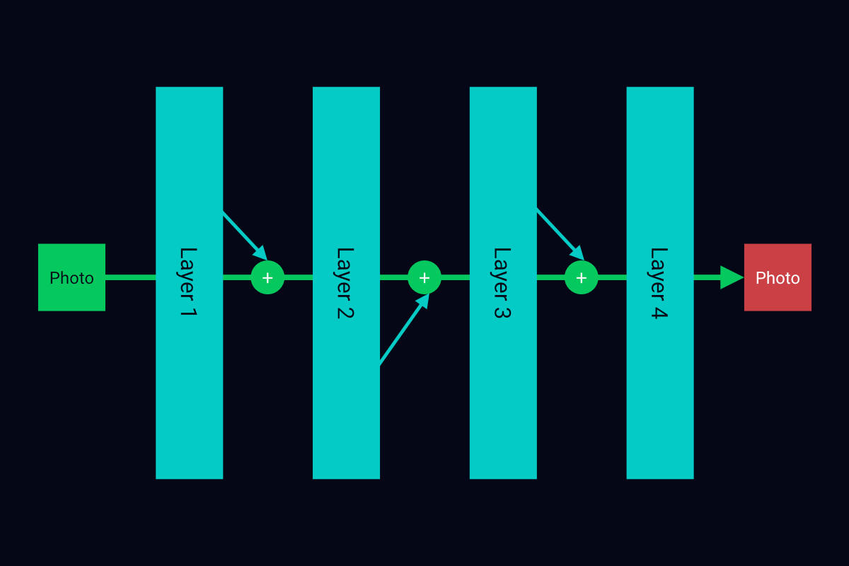
A ResNet representation
DenseNets are more recent than ResNets. DenseNets improve upon ResNets and can make more accurate predictions.
In a DenseNet model, each non-initial layer receives the concatenated outputs of all the layers that precede it. This means that, in addition to learning about features on its own, a DenseNet layer learns the features that each of its preceding layers had learned. Its acquired learning is not limited to the knowledge of only one predecessor.
The following figure is a representation of a DenseNet:
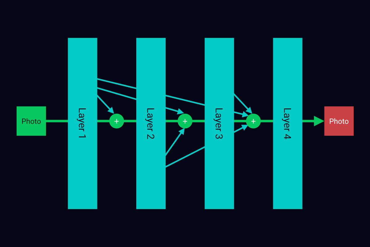
A DenseNet representation
For a video-based explanation of pretrained models, refer to the following YouTube content:
Now that we can distinguish between the pretrained models, let us get on the same page about how we will use each model.
Outlining the Process of Using Pretrained Models
Here are the broad-level steps that we will follow to classify images using the pretrained models:
- Create an initial file and folder structure for the project.
- Obtain the images.
- Convert each image into a format that pretrained models accept.
- Obtain a prediction about each image from the models.
Let us begin with the first step.
Step 1: Creating an Initial File and Folder Structure
In this step, we will set up an initial file and folder structure for the project in Google Drive. We will access the Google Drive home page, create a new folder in Google Drive, and add a new Google Colab notebook to the folder. As we progress through the project, we will save any additional project assets in this folder as well.
Once we have saved the Colab notebook, we will connect it to Google Drive—that is, mount Google Drive into the notebook. This will allow us to add other project assets to Google Drive from within the notebook, using code.
If you want to learn how to add a Colab notebook to a new Google Drive folder, connect the notebook to Google Drive, and run code in the notebook, watch the following video:
Once you have created the required project folder and notebook, move on to the second step. In this step, we will obtain six photos so that we can compare how accurately the models classify images.
If you prefer video to text, watch the following YouTube video as well. In this video, I use DenseNet201 to classify the image of a coyote. In doing so, I summarize all the subsequent steps (steps 2–4) of this project.
Step 2: Obtaining the Images
By default, each of the selected models can predict 1000 classes of day-to-day objects, including food items, animals, and birds. For this project, we will test the models on the photos of a tray of strawberries, a zebra, a flamingo, a pancake, a burger, and a car.
We will download the required photos from Unsplash using code. And we will run the code in the Colab notebook that we had created in Step 1.
To understand the code better, let us distribute it across the following five tasks:
- Create a file-path generator.
- Declare a photo-saving function.
- Create a destination folder.
- Make the destination path Python compatible.
- Download images and save them in the destination folder.
Here is the first task:
Task 1: Creating a File-Path Generator
In this task, we will declare a file-path generator. This function will automatically generate a valid file path, including a file name, for every image file that we download.
Each file path will point to the same storage location. In addition, the file name in each path will match a sequential pattern—for example, img_1.jpg, img_2.jpg, and img_3.jpg.
The function will work as follows:
Accept a storage location (folder path) and a file-naming pattern. The naming pattern will generate file names such as img_x.jpg, where x is a digit.
Initialize a counter.
Initialize a
whileloop.Within each pass of the loop, take the following actions:
a. Increment the counter by 1.
b. Generate a file path by combining the specified folder path and a file name. Base the file name on the provided naming pattern and the current counter value.
c. Check whether the file name in the generated path matches the name of any file that already exists in the specified folder.
d. If the file names exist, run another pass of the while loop using an incremented counter value. If the file name does not exist, return the generated file path.
Run the following code to declare the function:
def generate_file_path(destination, naming_pattern='img_{:d}.jpg'):
  counter = 0
  while True:
      counter += 1
      path = destination/naming_pattern.format(counter)
      if not path.exists():
          return path
Next, we will declare a function that can download photos and save them in one folder.
Task 2: Declaring a Photo-Saving Function
To add the photo-saving function to your notebook, run the following code:
# Importing a module that lets us retrieve
# content from web pages
import requests

# Specifying the function code
def save_image(url, destination):
  '''
  - Downloads image data via a URL request
  - Uses generate_file_path() to generate a file path
  - Saves image data using the generated file path
  '''
  # Making a request and retrieving image data
  img_data = requests.get(url).content

  # Generating a file path
  img_path = generate_file_path(destination)

  # Saving image data using the generated path
  with open(img_path, 'wb') as f:
      f.write(img_data)
Next, we will create a folder where we can save any downloaded images. We will create this folder at the same level as the project notebook.
Task 3: Creating a Destination Folder
The command to create the folder is give below. The command is based on the presumption that your project notebook is in a folder named deep-learning. The command will create a new folder named proj1_assets within the deep-learning folder.
These commands are based on the presumption that the notebook is in a Google Drive folder named deep-learning. The second command will create a new folder named proj2_assets within the deep-learning folder. We will unzip the compressed file into the proj2_assets folder.
If you saved the notebook in a different location, make sure you specify the correct path to the notebook after /content/drive/MyDrive/ in the following three commands.
!mkdir /content/drive/MyDrive/deep-learning/proj1_assets
Next, we will make sure we can download images using Pythonic code.
Task 4: Making the Destination Path Python Compatible
We cannot use the path to the destination folder as is in Pythonic code. This is because the path is in string format. To make the path Python compatible, we will have to convert it into a Path object. Run the following code to accomplish this task:
from pathlib import Path

base_path = '/content/drive/MyDrive/deep-learning/'
dest = Path(base_path + 'proj1_assets')
Finally, we will download and save images.
Task 5: Downloading and Saving Images
In this task, we will put the save_image function and the Path instance to use.
Here is the code that you need to run in your notebook:
# Downloading and saving an image of strawberries
save_image('https://source.unsplash.com/YrGa20k9Coo/224x224', dest)

# Downloading and saving an image of a zebra
save_image('https://source.unsplash.com/c_cPNXlovvY/224x224', dest)

# Downloading and saving an image of a flamingo
save_image('https://source.unsplash.com/wTPp323zAEw/224x224', dest)

# Downloading and saving an image of a pancake
save_image('https://source.unsplash.com/t6xh7hskUVA/224x224', dest)

# Downloading and saving an image of a burger
save_image('https://source.unsplash.com/dphM2U1xq0U/224x224', dest)

# Downloading and saving an image of a car
save_image('https://source.unsplash.com/pr-Zr7YHFy0/224x224', dest)
Now, we can move on to the second step in the process of using pretrained models.
Step 3: Converting Each Image into an Acceptable Format
In this step, we will write a function that can apply the following changes to each image:
Load the image in the Pillow (PIL) format. A PIL image is compatible with Pythonic code. We will use the
load_imgfunction of theimagemodule oftensorflow.keras.preprocessingto change the format of the image to PIL and load the image.Convert the loaded image into a NumPy array. This conversion will make the image compatible with
keras. We will use theimg_to_arrayfunction of theimagemodule to convert each image.Expand the array version of the image from three dimensions to four dimensions. The fourth dimension will indicate the number of images per input. The expansion is necessary because a model can accept multiple images per pass, while we will supply only one image in each pass.
The unexpanded version of each of our downloaded images has the shape 224 x 224 x 3. In this shape format, the first two numbers represent the width and height of the image and the last number represents the number of color channels in the image (RGB in this project). After expansion, the image will have the shape 1 x 224 x 224 x 3, where 1 indicates the number of images per input.
Modify each expanded image so that it has the same format as the sample data1 of the pretrained model that we have chosen for image identification. We will use the
preprocess_inputfunction that comes out of the box with every pretrained model to apply the modifications.
To apply the changes, we will first import the image module and the modules that make each model’s preprocess_input function available to us. Run the following code to import the modules:
# Importing modules
from tensorflow.keras.preprocessing import image
from tensorflow.keras.applications import resnet, densenet
Next, run the following code to declare the custom function.
# Declaring custom function
def convert_image(img, model_type):
  loaded_img = image.load_img(img)
  img_arr = image.img_to_array(loaded_img)
  if 'resnet' in model_type:
      processed_img = resnet.preprocess_input(\
      img_arr.reshape((1, 224, 224, 3)))
  elif 'densenet' in model_type:
      processed_img = densenet.preprocess_input(\
      img_arr.reshape((1, 224, 224, 3)))
  else:
    print('''The model_type string should
        include either of the following words:
        resnet or densenet''')
    return
  return loaded_img, processed_img
We will run the convert_image function in the next step.
Step 4: Obtaining Predictions from Each Pretrained Model
In this step, we will perform the following tasks:
- Save the path to each of the six images in a list.
- Write a function that can obtain predictions about all the six images at once from a specific model.
- Use the function to obtain predictions from the three models.
Task 1: Saving Image Paths in a List
Here is the code for this task:
# Retrieving the paths to all JPG images in the
# proj1_assets folder and saving the paths in a list
import glob
images = []
image_paths = base_path + "proj1_assets/*.jpg"

for file_name in glob.glob(image_paths):
  images.append(file_name)
Task 2: Declaring a Prediction-Display Function
This function will accept three arguments, which are described below:
The first two arguments will be variables that specify model instance and model type. We had discussed constraints pertaining to the latter variable,
model_type, in the previous step.The third argument will specify the number of predictions we want to retrieve per image. We will use the model-specific
decode_predictionsfunction ofkerasto retrieve the predictions.The
decode_predictionsfunction can convert its corresponding models’ predictions from exponential numbers to human friendly alphanumeric characters. In addition, by default, this function can retrieve the top-five predictions of its model. We will obtain only the top-three predictions, however.
Here is code related to the prediction-display function:
# Importing models
from tensorflow.keras.applications import ResNet50,\
DenseNet121, DenseNet201

# Importing a matplotlib module that will let us
# display images as well as predictions about them
import matplotlib.pyplot as plt

# Configuring the display style of matplotlib
plt.style.use("dark_background")

# Declaring the custom function
def get_prediction(model_instance, model_type, num_pred=3):
  # Setting the overall image-display area
  plt.figure(figsize=(15,10))

  # Making the model_type string lowercase
  model_type = model_type.lower()

  # Using a for loop to process each image and
  # display related predictions
  for i in range(6):
    # Generating a subplot at index (i+1) in a
    # grid of 2 rows and 3 columns
    plt.subplot(2,3,i+1)

    # Making sure the model_type string contains a valid value
    # Displaying a message and exiting function if
    # valid value not present
    if 'resnet' not in model_type:
      if 'densenet' not in model_type:
        print('''The model_type string should
        include either of the following words:
        resnet or densenet''')
        return

    # Using the convert_image function to
    # process the current image
    try:
      loaded_img, processed_img = convert_image(images[i], model_type)
    except Exception as e:
      print(e)
      return

    # Generating prediction
    prediction = model_instance.predict(processed_img)

    # Converting the models' predictions from exponential
    # numbers to human friendly alphanumeric characters and
    # obtaining a specific number of predictions (num_pred)
    # As decode_predictions returns a list within a list,
    # extracting the inner list ([0]) as well
    try:
      if 'resnet' in model_type:
        decoded_preds = resnet.decode_predictions(prediction, top=num_pred)[0]
      if 'densenet' in model_type:
        decoded_preds = densenet.decode_predictions(prediction, top=num_pred)[0]
    except Exception as e:
      print(e)
      return

    # Extracting predicted classes and the likelihood of the
    # image belonging to each class
    pred_vals=''
    for i in range(num_pred):
      pred_vals += decoded_preds[i][1].capitalize()\
        + ' ' + str(round(decoded_preds[i][2]*100, 2)) + '%'
      if i<2:
        pred_vals += '\n'

    # Displaying the current image
    plt.imshow(loaded_img)

    plt.grid(False)
    plt.subplots_adjust(left=0.12,
                    bottom=0.1,
                    right=0.9,
                    top=0.9125)
    plt.xticks([])
    plt.yticks([])

    # Making sure the consolidated predictions about the image
    # are displayed in its title
    plt.title(pred_vals,size=16,ha='center',y=1.01)

  # Specifying that the final output should be saved as a
  # png file that is named after the current model type
  plt.savefig(base_path + model_type + '.png',\
              facecolor='#0a0a0a',edgecolor='none',bbox_inches='tight')
Let us implement the function now.
Task 4: Obtaining Predictions from the Three Models
We will obtain predictions one by one from ResNet50, DenseNet121, and DenseNet201.
ResNet50 Predictions
Here is the code that we will use to obtain predictions from ResNet50:
# Creating a ResNet50 instance
model_instance = ResNet50()

# Displaying predictions
get_prediction(model_instance, 'resnet')
And here is the output of the code:
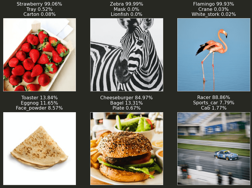
The top-three predictions of ResNet50
DenseNet121 Predictions
To get predictions form DenseNet121, we will run the following code:
# Creating a DenseNet121 instance
model_instance = DenseNet121()

# Displaying predictions
get_prediction(model_instance, 'densenet121')
Here is the output of the code:

The top-three predictions of DenseNet121
DenseNet201 Predictions
For DenseNet201 predictions, we will run the following code:
# Creating a DenseNet201 instance
model_instance = DenseNet201()

# Displaying predictions
get_prediction(model_instance, 'densenet201')
Here is the output of the code:

The top-three predictions of DenseNet201
Conclusion
In this project, we used three pretrained TensorFlow models to classify six images. Each model could classify all the images except one—the image of a pancake—correctly, with an acceptable prediction probability.
Among the three models, DenseNet201 exhibited the best performance. Its prediction probability was 91.64% or more for five of the images.
Sample data is the data on which a production version of a model had been trained. ↩︎